Diffusion model from scratch
Denoising diffusion probabilistic (opens in a new tab) models are behind many popular image/audio generation apps such as: Stable Diffusion (opens in a new tab), Midjourney (opens in a new tab), Dall-E (opens in a new tab), and Imagen (opens in a new tab).
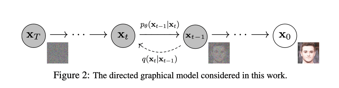
Q: Why can both processes be defined as parametrized Markov chains?
A: Because each circle is a whole distribution and then there is a "line" from each point in the distribution to each point distribution representing the probability of transition.
Most ML folks have a surface understanding of diffusion models and simply think about it as follows: During training there is a forward process and a backwards process . takes an image and gradually adds gaussian noise in steps. takes the output of after steps and tries to gradually reconstruct the original image. We aim for distributions and (where is the step) to be the same, and that's what we compute the loss with respect to. Finally, once the training is done and loss is minimizes, we need only the process for the inference. will take any random gaussian noise as input and produce some meaningul image.
That sounds simple right? And this is the correct way to understand the abstract concept of diffusion models. But my curious mind didn't give me rest so questions kept popping up in my head:
- How do we measure the distance between two distributions and how do we minimize it?
- How complex does the model that predicts denoising need to be ?
- How can forward process add meaningful features and produce a real image from Gaussian noise?
You can only fully understand how something works if you build it yourself. So I read up on various blogs and papers: 1 (opens in a new tab), 2 (opens in a new tab),3 (opens in a new tab), 4 (opens in a new tab), 5 (opens in a new tab) and started implementing diffusion model myself.
For a full implementation see my Google Colab notebook https://colab.research.google.com/drive/14UJQ6LTKPo4RgQT-kSjpswkI7Q1oYPW4 (opens in a new tab), here I will explain each code snippet.
def sample_batch(size,noise=1.0):
    x , _=make_swiss_roll(size, noise=noise)
    # we want it in 2d so we take 0th and 2nd coord
    return x[:, [0,2]] / 10.0
data = sample_batch(10**4).T
First, we will focus on the swiss roll dataset. The aim is for the forward process to learn to generate points that belong to the swiss roll. Therefore, if we randomly sample many points using pretrained we will construct swiss roll distribution. In the code snippet above we use sklearn's function to sample data points, and take coordinates x and z ([x:, [0,2]]), since by default sklearn creates 3D swiss roll. We could've also just defined the dataset ourselves, since the swiss roll in 2D is defined by a map
start=1e-5
end=1e-2
n_steps=100
betas = torch.sigmoid(torch.linspace(-6, 6, n_steps)) * (end-start)+start
alphas = 1 - betas
alphas_bar = torch.cumprod(alphas, 0)
This code snippet is essentially defining required variables, but there is a lot to unpack here.
Forward process is defined by the formula
Here we sample a point that is similar to the point in the previous step but with some noise induced. I think of this as: "remove some small part and add random noise in it's place. Betas are hyperparameters and they represent the noise schedule, the higher betas are the faster we will induce the noise, note that they have to be between zero and one. We select the sigmoid schedule above because it worked the best in our experiments.
But with the above formula, we cannot directly calculate , we would have to calculate points first. It would be neat if we can get it in . In the denoising diffusion paper, they simpify the formula to:
where
With this we achieve much faster compute time.
Next, we define a model that will predict denoising. The reverse process is defined as:
where and are uknown, and is what we need the model to predict.
In the denoising diffusion models paper, they further simplify this process to rely only on the function by defining mean as:
and using a fixed variance function instead. This results in the following sampling equation:
where
Therefore, our model needs to learn only the function
class ConditionalLinear(nn.Module):
    def __init__(self, num_in, num_out, num_classes):
        super().__init__()
        self.num_out = num_out
        self.lin = nn.Linear(num_in, num_out)
        self.embed = nn.Embedding(num_classes, num_out)
        #used to initialize weights of the embedding layer to
        #the values drawn from uniform distribution
        self.embed.weight.data.uniform_()

    def forward(self, x, y):
        out = self.lin(x)
        gamma = self.embed(y)
        out = gamma.view(-1, self.num_out) * out
        return out

class ConditionalModel(nn.Module):
    def __init__(self, n_steps):
        super(ConditionalModel, self).__init__()
        self.lin1 = ConditionalLinear(2, 128, n_steps)
        self.lin2 = ConditionalLinear(128, 128, n_steps)
        self.lin3 = ConditionalLinear(128, 128, n_steps)
        # only two outs
        self.lin4 = nn.Linear(128, 2)

    def forward(self, x, y):
        x = F.softplus(self.lin1(x, y))
        x = F.softplus(self.lin2(x, y))
        x = F.softplus(self.lin3(x, y))
        return self.lin4(x)
For our architecture, we will simply use a stack of linear layers with the softplus activation function. However,
since we are going to use the same set of weights to predict each transition, we need to condition the model on the number of steps.
So instead of simply using a linear layer we define a conditional linear layer.
For each step each layer will learn a vector corresponding to the number of steps
(nn.Embedding(num_classes, num_out))
,and then multiply the output by this vector to condition it:
out = gamma.view(-1, self.num_out) * out
The output of the last layer has only 2 numbers - namely values of two-dimensional value . Next, it's time to talk about the loss.
def noise_estimation_loss(model, x0):
    batch_size = x0.shape[0]
    t = torch.randint(0, n_steps, size=(batch_size,)).long()
    e = torch.randn_like(x0)
    #broadcast
    x = x0 * torch.sqrt(alphas_bar[t]).unsqueeze(1) + e * torch.sqrt(1-alphas_bar[t]).unsqueeze(1)
    output = model(x, t)
    return (e - output).square().mean()
The above code snippet might be the most complicated bit to understand. To fully understand how we got the noise estimation loss we would need to do a lot of math, but for now I will try to explain the intuition behind it and leave it to the reader to check the math in the original paper. With generative models, we usually optimize the variational bound on negative log likelihood. In other words, we want to find what is the probability of observing the data given the set of weights, and find a set of weights that maximizes this likelihood.
The probability that diffusion model assigns to the data is:
(joint probability of the entire trajectory)
and then we want to minimize
Now, authors of denoising diffusion paper simplify this objective, and obtain the following loss:
One other term that might not be clear in the snippet above is t. We randomly choose a step at which we want to compute the loss for each element in the batch. For that step we compute the difference between and distribution. Or in other words, we want the distribution obtained after adding noise in steps to be the same as the distribution after removing noise in steps.
def get_pt(x,t):

    t = torch.tensor([t])
    eps_factor = (1 - alphas[t]) / torch.sqrt(1-alphas_bar[t])
    eps_theta = model(x, t)
    mean = 1 / (alphas[t].sqrt()) * (x - (eps_factor * eps_theta))
    z = torch.randn_like(x)
    sigma_t = betas[t].sqrt()
    sample = mean + sigma_t * z
    return sample

def p_sample_loop(shape):
    cur_x = torch.randn(shape)
    x_seq = [cur_x]
    for i in reversed(range(n_steps)):
        cur_x = get_pt(cur_x, i)
        x_seq.append(cur_x)
    return x_seq
We defined functions to sample a point from the learned distribution using this formula.
model = ConditionalModel(n_steps)
optimizer = optim.Adam(model.parameters(), lr=1e-3)
dataset = torch.tensor(data.T).float()
batch_size = 128
for t in range(1000):
    permutation = torch.randperm(dataset.size()[0])
    for i in range(0, dataset.size()[0], batch_size):
        indices = permutation[i:i+batch_size]
        batch_x = dataset[indices]

        loss = noise_estimation_loss(model, batch_x)
        optimizer.zero_grad()
        loss.backward()
        torch.nn.utils.clip_grad_norm_(model.parameters(), 1.)
        optimizer.step()

    if (t % 100 == 0):
        print(loss)
Finally, we train the model. We use Adam optimizer, batch size of and clip gradients at 1.
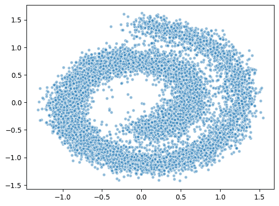
x_seq = p_sample_loop(dataset.shape)
plt.scatter(*x_seq[-1].T.detach().numpy(), alpha=0.5, edgecolor='white', s=20)
Visualize the learned distribution.